Taiga.jl

Tensor-product applications in isogeometric analysis.

Note

Examples listed on this page use following packages

using Taiga
using LinearAlgebra
using SortedSequences, CartesianProducts, KroneckerProducts, NURBS, SpecialSpaces, AbstractMappings, UnivariateSplines

Postprocessing

Some basic postprocessing methods are provided as Plots recipes in most packages in the Feather ecosystem. Taiga.jl implements Bézier extraction and can save mappings, fields and control nets to a VTK file, e.g

mapping = hole_in_square_plate()
mapping = refine(mapping, method=hRefinement(3))
space = ScalarSplineSpace(mapping.space)

euclidean_distance = Field((x,y) -> sqrt(x^2 + y^2))
d = Field(space)
project!(d, onto=euclidean_distance ∘ mapping; method=QuasiInterpolation)

vtk_save_bezier("geometry_and_field", mapping; fields = Dict("d" => d))
vtk_save_control_net("control_net", mapping)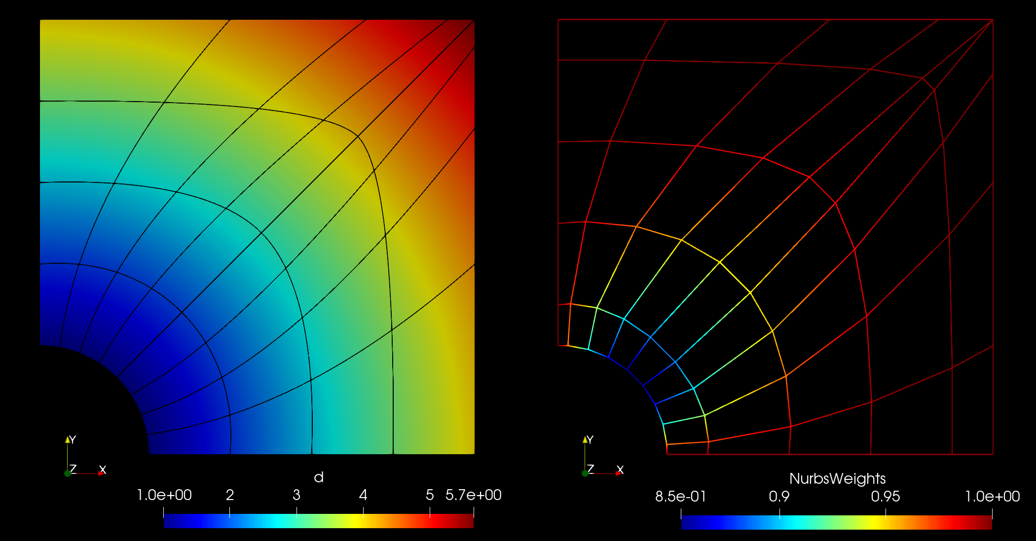

Bezier extraction on square plate with a hole

More detailed examples are provided in the examples directory.

Aggregation of Kronecker products

More often then not Kronecker product approximations will be composed of a sum of Kronecker products. In most cases these sums will not have the classical Kronecker sum structure. Nonetheless, it is still possible to evaluate matrix-vector products with these operators with complexity $\mathcal O(M\cdot N^{3/2})$ and $\mathcal O(M\cdot N^{4/3})$ in 2 and 3 dimensions, where $M$ is the number of Kronecker products in the collection.

KroneckerProductAggregate is a collection of Kronecker product matrices of conforming size that acts as a linear map and supports reduction over the collection, e.g.

julia> A = rand(7, 3) ⊗ rand(5, 3) ⊗ rand(3, 5);

julia> B = rand(7, 3) ⊗ rand(5, 3) ⊗ rand(3, 5);

julia> C = A + B;

julia> K = KroneckerProductAggregate(A, B);

julia> v = rand(size(C, 2));

julia> b = K * v;

julia> b ≈ C * v
true

julia> mul!(b, K, v); # in-place evaluation

julia> b ≈ C * v
true

A KroneckerProductAggregate supports LinearAlgebra.mul!, LinearAlgebra.adjoint, Base.isempty, Base.push! and most other methods that abstract matrices implement.

`KroneckerFactory`

Let us consider that we need to assemble the bilinear form associated with the operator L(u) = ∇ ⋅ (C∇u) where C = [6.0 0.1875; 0.125 12.0] is a conductivity matrix. Clearly, even on Cartesian grids an exact FastDiagonalization of the resulting matrix is not possible due to non-zero off-diagonal entries in C. Furthermore, if C is a function of the spatial coordinates, the resulting stiffness matrix does not have a Kronecker product structure at all and the material pullback needs to be approximated using some separable approximation.

KroneckerFactory can be used to obtain approximations of a bilinear form given a separable approximation of the data, i.e. weighted spline approximation of the pullback operator on mapped geometries or Wachspress approximation at quadrature points.

The syntax is close to that of IgaFormation.Sumfactory.

# domain
Ω = Interval(0.0, 1.0) ⨱ Interval(0.0, 1.0)

# partition
Δ = Partition(Ω, (3,5))

# space
p = (2,3)
S = ScalarSplineSpace(p, Δ)

# mock data
Dim = length(S)
nqpts = map((p,n) -> (p+1)*n + 2, p, num_elements.(S))
f = [ map(rand, nqpts) for k ∈ 1:Dim, l ∈ 1:Dim]

# derivative indicators
∇u = k -> ι(k, dim=Dim)
∇v = k -> ι(k, dim=Dim)

# assemble stiffness
∫ = KroneckerFactory(S, S)
for β in 1:Dim
    for α in 1:Dim
        ∫(∇u(α), ∇v(β); data=f[α, β])
    end
end

# aggregated Kronecker products
K = ∫.data

In the above, f[α, β] is a Tuple of either univariate weighting splines in each parametric direction or plain vectors with weighting coefficients. This data is used to weight the test functions.

Similarly to Sumfactory, the data collection can be reset

∫(∇u(α), ∇v(β); data=f[α, β], reset=true)

or simply

reset!(∫)

Linear solvers

Taiga provides minimal reference implementations of linear solvers:

TaigaCG Conjugate Gradient method
TaigaPCG preconditioned Conjugate Gradient method
TaigaIPCG inexactly preconditioned Conjugate Gradient method

These implementations are reasonably fast. The solution times are at least as good as Krylov.jl, whereby due to the minimal implementation there are less memory allocations. Furthermore, some solvers like TaigaIPCG are nowhere to be found and are essential to Taiga's conceptual framework.

julia> solver = TaigaPCG(L, P; atol=10e-8, rtol=10e-8, itmax=100)
Linear solver of type TaigaPCG (atol=1.0e-7, rtol=1.0e-7, itmax=100)

julia> x, stats = linsolve!(solver, b);

julia> stats
Linear solver statistics for TaigaPCG:
┌──────────────────┬───────────────────────────────┐
│ Metric           │ Value                         │
├──────────────────┼───────────────────────────────┤
│ converged        │ true                          │
│ niter            │ 47                            │
│ residual_norm    │ 9.25797e-8                    │
│ residual_norm_x₀ │ 0.0732086                     │
│ status           │ coverged: atol ✔, rtol ✘      │
└──────────────────┴───────────────────────────────┘

Index

Taiga.BezierExtractionContext — Type

BezierExtractionContext{Dim, T}

Bezier extraction context.

Fields:

splinespace::TensorProduct{Dim, SplineSpace{T}}: spline space
partition::CartesianProduct{Dim}: partition
C::Array{KroneckerProduct, Dim}: Bezier extraction operators
bezier_basis_dimension::NTuple{Dim}: Bezier basis dimension

References

- Gene H. Golub and Qiang Ye. Inexact preconditioned conjugate gradient method with inner-outer iteration. SIAM J. Sci. Comput., 21(4):1305–1320, December 1999.
- Andrew V Knyazev and Ilya Lashuk. Steepest descent and conjugate gradient methods with variable preconditioning. SIAM Journal on Matrix Analysis and Applications, 29(4):1267–1280, 2008.
Taiga.TaigaPCG — Type
TaigaPCG{T, L, P}Linear solver implementing the preconditioned Conjugate Gradient method.
Taiga.TargetSpace — Type
const TargetSpace{T} = UnivariateSplines.SplineSpace{T}Alias for UnivariateSplines.SplineSpace.
Taiga.TestSpace — Type
const TestSpace{T} = UnivariateSplines.SplineSpace{T}Alias for UnivariateSplines.SplineSpace.
Taiga.VTKHigherOrderDegrees — Type
VTKHigherOrderDegrees{Dim, T}An immutable sparse container for WriteVTK higher order degrees array.
This container acts like an array of size (3, ncells) with repeated columns and supports indexing and views.
Fields:
degrees::NTuple{Dim, T}: cell degreesncells::Int: number of Bezier cells
Taiga.Wachspress — Type
ModalSpline <: DataApproximationMethodMethod to approximate patch data at quadrature points using Wachspress algorithms. Works only for data arrays with positive entries.
Base.adjoint — Method
LinearAlgebra.adjoint(K::KroneckerProductAggregate)Returns an adjoint KroneckerProductAggregate.
Base.getproperty — Method
Base.getproperty(A::LinearSolverStatistics, field::Symbol)Returns field in A (actually the value associated with key field in A.data).
Base.propertynames — Method
Base.propertynames(A::LinearSolverStatistics)Returns all property names of A (keys in A.data!).
Base.push! — Method
Base.push!(K::KroneckerProductAggregate{T}, k::S) where {T,S<:KroneckerProduct{T}}Adds a Kronecker product matrix to the collection of Kronecker products in K.
Base.setproperty! — Method
Base.setproperty!(A::LinearSolverStatistics, field::Symbol, value)Sets field in A (actually A.data[field]) to value.
Arguments:
A: statistics containerfield: field to set (a key indata)value: value to set
LinearAlgebra.isposdef — Method
LinearAlgebra.isposdef(P::H)Returns true if σ(inv(P₀)A) ⊂ (0,2) and false otherwise.
LinearAlgebra.opnorm — Method
LinearAlgebra.opnorm(A::K) where {Dim,T<:Real,K<:KroneckerProduct{T,2,Dim}}Returns the operator norm ‖A‖₂ of a Kronecker product using Kronecker product eigenvalue decomposition of AᵀA which is fast.
Taiga.apply_particular_solution — Function
apply_particular_solutionEach model module implements its own method for apply_particular_solution, which adds particular solution to homogeneous solution.
Taiga.approximate_patch_data — Function
approximate_patch_dataMethods implementing patch data approximation algorithms.
Taiga.approximate_patch_data — Method
approximate_patch_data(C::E, args; method::Type{<:DataApproximationMethod}, kwargs) where {S1,S2,E<:EvaluationSet{S1,S2}}Approximate patch data using method. Calls implementation of approximation_patch_data for method with positional arguments args and keyword arguments kwargs.
C: patch data asIgaFormation.EvaluationSetargs: positional arguments to methodmethod: approximation methodkwargs: keyword arguments to method
approximate_patch_data(::Type{<:CanonicalPolyadic}, C::E; tol::T=10e-1, rank::Int=1, ntries::Int=10) where {Dim,S1,S2,E<:EvaluationSet{S1,S2},T}Returns an array of size rank × S1 × S2 of Vector tuples of length Dim for each data array in C.
C: patch data asIgaFormation.EvaluationSettol: cp tolerancerank: number of cp modesntries: number of attempts to compute the CP decomposition per block
approximate_patch_data(::Type{<:ModalSplines}, C::E; S::NTuple{Dim,SplineSpace{T}}, rank::Int=1) where {Dim,S1,S2,E<:EvaluationSet{S1,S2},T}Returns an array of size rank × S1 × S2 of Bspline tuples of length Dim for each data array in C.
C: patch data asIgaFormation.EvaluationSetspaces: tuple of univariate interpolation spline spacesrank: approximation rank
Taiga.bezier_basis_dimension — Method
bezier_basis_dimension(S::TensorProduct{Dim, SplineSpace{T}})Returns Bezier basis dimension if extracted from S.
Taiga.droptol! — Method
droptol!(K::S; rtol = √(eps(T)))Drop contributions in K = {K₁, K₂, ...} for which the relative operator norm ‖Kₖ‖₂ / || ‖Kₘₐₓ‖₂ is less then rtol, where for Kₖ ∈ K we find Kₘₐₓ = argmax ‖Kₖ‖₂.
Taiga.extreme_eigenvalues — Method
extreme_eigenvalues(A::L; tol::T = 0.1, restarts::Int=200) where {T,L<:LinearMap}Compute extreme eigenvalues of a linear map A. Uses ArnoldiMethod. The tolerance tol can be helpful if ArnoldiMethod converges to more then one maximum or minimum eigenvalue. Checks for complex eigenvalues are performed.
Taiga.forcing — Function
forcingEach model module implements its own method for forcing, which returns the right hand side vector.
Taiga.forcing! — Function
forcing!Each model module implements its own method for forcing!, which updates the right hand side vector.
Taiga.get_bezier_basis_indices — Method
get_bezier_basis_indices(S::SplineSpace, e::Integer)Computes univariate basis indices of a Bezier basis corresponding to Bspline space S.
Taiga.get_system_matrix_quadrule — Method
get_system_matrix_quadrule(S::TargetSpace, V::TestSpace)Returns a univariate PatchRule for a pair of spaces.
Taiga.hyperpower_eigenvalues_after_n_iterations — Method
hyperpower_eigenvalues_after_n_iterations(λ::T; n::Int)For a set of eigenvalues λ return the corresponding eigenvalues after n further updates of the Ben-Israel-Cohen iteration.
Transformation rule applies for λ after first update. The upper bound for λ after first update is 1.
Example:
julia> λ₀ = hyperpower_extreme_eigenvalues(P; n=0, tol=10e-5)
(0.023145184193109333, 1.9749588237991926)
julia> λ₁ = hyperpower_extreme_eigenvalues(P; n=1, tol=10e-5)
(0.045754651575638426, 0.9999899575917253)
julia> hyperpower_extreme_eigenvalues(P; n=5, tol=10e-5)
(0.5273271247385951, 0.9999962548752878)
julia> hyperpower_eigenvalues_after_n_iterations(λ₁; n=4)
(0.5273268941262143, 1.0)
julia> hyperpower_eigenvalues_after_n_iterations(λ₀; n=1)
(0.0457546604483684, 0.049592390484542115)Taiga.hyperpower_extreme_eigenvalues — Method
hyperpower_extreme_eigenvalues(P::H; n::Int=1, tol::T=√eps(T)) where {Dim,T,H<:HyperPowerPreconditioner{Dim,T}}Compute the extreme eigenvalues of inv(Pₙ)A, i.e. return a tuple (λmin, λmax) in nth iteration.
In the case of eigenvalue clustering, i.e. around the value of 1, it might be necessary to choose lower tol.
julia
julia> hyperpower_extreme_eigenvalues(P; n=2, tol=10e-5)
(0.08941582990237358, 0.9999916150622586)
julia> hyperpower_extreme_eigenvalues(P; n=3, tol=10e-5)
(0.1708364549356042, 1.0000016638364837)
julia> hyperpower_extreme_eigenvalues(P; n=4, tol=10e-5)
(0.3124877477755778, 0.9999984021406245)
julia> hyperpower_eigenvalues_after_n_iterations(λ₁; n=2)
(0.17083641016503434, 1.0)
julia> hyperpower_eigenvalues_after_n_iterations(λ₁; n=3)
(0.31248774129199286, 1.0)
(0.0457546604483684, 0.049592390484542115)Taiga.hyperpower_initial_preconditioner — Method
hyperpower_initial_preconditioner(P::H)Returns the initial preconditioner that was used in the construction of P, e.g. FastDiagonalization.
Taiga.inner_solver_convergence — Method
inner_solver_convergence(P::S) where {S<:Union{InnerCG, InnerPCG}}Returns a vector booleans indicating convergence in last applications of InnerPCG preconditioner.
See reset_inner_solver_history! to reset history.
Taiga.inner_solver_niters — Method
inner_solver_niter(P::S) where {S<:Union{InnerCG, InnerPCG}}Returns a vector with numbers of iterations in last applications of InnerCG and InnerPCG preconditioner.
Taiga.inner_solver_residuals — Method
inner_solver_residuals(P::S) where {S<:Union{InnerCG, InnerPCG}}Returns a vector with residuals in last applications of InnerPCG preconditioner. See reset_inner_solver_history! to reset history.
Taiga.linear_operator — Function
linear_operator()Returns a linear operator for a model. Each model module implements this.
Taiga.linear_operator_approximation — Function
linear_operator_approximation()Returns a linear operator approximation for a model. Some model modules implements this. Linear operator approximations are cheap to apply and useful in the context of preconditioning.
Taiga.linsolve! — Function
linsolve!Linear solvers implement this method. Typically, the syntax is linsolve!(solver, rhs; kwargs...)
Taiga.linsolve! — Method
linsolve!(solver::TaigaCG{T, L}, b::Vector{T}; x0::Vector{T} = zeros(size(solver.A, 2)))Solve the linear system A x = b using TaigaCG.
solver: solver contextb: rhs vectorx0: initial guess
linsolve!(solver::TaigaCG{T, L}, b::Vector{T}; x0::Vector{T} = zeros(size(solver.A, 2)))Solve the linear system A x = b using TaigaIPCG.
linsolve!(solver::TaigaPCG{T, L}, b::Vector{T}; x0::Vector{T} = zeros(size(solver.A, 2)))Solve the linear system A x = b using TaigaPCG.
Taiga.reset! — Method
reset!(f::KroneckerFactory)Reset KroneckerProductAggregate collection in KroneckerFactory.
Taiga.reset_inner_solver_history! — Method
reset_inner_solver_niter_history!(P::S) where {S<:Union{InnerCG, InnerPCG}}Taiga.system_matrix_integrand — Method
system_matrix_integrand(S::TargetSpace{T}, V::TestSpace{T}, k::Int = 1, l::Int = 1; x::T)Evaluates to the integrand of a system matrix ∫ s(ξ)v(ξ) dΩ for ξ = x where s ∈ S and v ∈ V.
This is useful i.e. in the definition of boundary integrals on Cartesian grids.
S: aUnivariateSplines.SplineSpaceas target spaceV: aUnivariateSplines.SplineSpaceas test spacek: derivative order on target spacel: derivative order on test spacex: evaluation point
Taiga.update_linear_solver_statistics! — Method
update_linear_solver_statistics!(solver::S)For η = √rᵀr and η₀ = √r₀ᵀr₀ and check η < atol, η₀ < rtol and if number of iterations is equal to itmax. Sets solver.stats.converged and solver.stats.status accordingly.
Taiga.vtk_bezier_cell_degree — Method
vtk_bezier_cell_degree(S::BezierExtractionContext{Dim, T}) where {Dim,T<:SplineSpace}Computes univariate degrees for a Bezier cell in a BezierExtractionContext.
vtk_bezier_cell_degree(S::TensorProduct{Dim, T}) where {Dim,T<:SplineSpace}Computes a tuple of univariate degrees for a Bezier cell extracted from a tensor product spline space.
Taiga.vtk_bezier_cells — Method
vtk_bezier_cells(B::VTKBezierExtractionContext)Collects all Bezier cells in B.
Taiga.vtk_bezier_degrees — Method
vtk_bezier_degrees(B::VTKBezierExtraction)Returns an immutable sparse array container of type VTKHigherOrderDegrees with cell degrees.
Taiga.vtk_cell_connectivity — Method
vtk_cell_connectivity(B::BezierExtractionContext{Dim, T})Returns cell connectivity for a BezierExtractionContext.
Taiga.vtk_cell_point_indices — Method
vtk_cell_point_indices(order::NTuple{Dim, Int}) where {Dim}Computes point indices of a reference VTK Bezier cell with points indexed using Cartesian indices.
Taiga.vtk_cell_type — Method
vtk_cell_type(::VTKBezierExtraction{Dim}) where {Dim}Returns a Bezier cell type based on Dim.
Taiga.vtk_control_net_cells — Method
vtk_control_net_cells(connectivity::Vector{Tuple{Int, Int}})Returns a vector of VTKCellTypes.VTK_LINE cells given a vector of point connectivities.
Taiga.vtk_control_net_connectivity — Method
vtk_control_net_connectivity(mapping::GeometricMapping{Dim})Generates a list of connectivity tuples for all edges of a control net based on the size of the control points grid in mapping.
Taiga.vtk_control_net_points — Method
vtk_control_net_points(mapping::GeometricMapping{Dim, Codim})Returns vectorized NURBS coefficients (for WriteVTK purposes).
Taiga.vtk_control_net_weights — Method
vtk_control_net_weights(mapping::GeometricMapping)Returns vectorized NURBS weights (for WriteVTK purposes).
Taiga.vtk_extract_bezier_points — Method
vtk_extract_bezier_points(B::BezierExtractionContext{Dim}, F::Field{Dim, Codim})Returns Bezier points of a Bspline field.
vtk_extract_bezier_points(B::BezierExtractionContext{Dim}, F::GeometricMapping{Dim, Codim}; bezier_weights = nothing, vectorize = true)Returns Bezier weights from a NURBS geometric mapping.
If vectorize is true the result is a tuple of vector views to the points.
Precomputed Bezier weights can be passed in bezier_weights explicitly. If not provided, these will be computed automatically.
vtk_extract_bezier_points(B::BezierExtractionContext{Dim}, F::M) where {Dim,Codim,M<:AbstractMapping}Returns Bezier points of Galerkin projection of an abstract mapping.
Consider this a fallback routine: it is used only if the mapping F is not a B-spline or NURBS map.
vtk_extract_bezier_points(B::BezierExtractionContext{Dim, T}, bezier_weights::Array{T, Dim}, spline_weights::Array{T, Dim}, spline_coeffs::Array{T, Dim})Returns Bezier points from NURBS control points.
vtk_extract_bezier_points(B::BezierExtractionContext{Dim, T}, spline_coeffs::Array{T, Dim})Returns Bezier points from Bspline control points (i.e. without rational weighting).
Taiga.vtk_extract_bezier_weights — Method
vtk_extract_bezier_weights(B::BezierExtractionContext{Dim}, F::GeometricMapping{Dim, Codim})Returns Bezier weights from a NURBS geometric mapping.
vtk_extract_bezier_weights(B::BezierExtractionContext{Dim, T}, spline_weights::Array{T, Dim})Returns Bezier weights from NURBS weights.
Taiga.vtk_map_linear_indices — Method
vtk_map_linear_indices(lind::AbstractArray, connectivity::NTuple{N, Int}) where {N}Maps linear indices of a Bezier cell index by Cartesian indices based on the connectivity of a reference VTK Bezier cell.
Taiga.vtk_num_cell_vertices — Method
vtk_num_cell_vertices(B::BezierExtractionContext)Returns number of vertices.
Taiga.vtk_num_cells — Method
vtk_num_cells(B::BezierExtractionContext)Returns number of Bezier cells.
Taiga.vtk_point_index_from_ijk — Method
vtk_point_index_from_ijk(inds::CartesianIndex{1}, order::NTuple{2, Int})Computes VTK point index based on Cartesian index of a cell point.
vtk_point_index_from_ijk(inds::CartesianIndex{2}, order::NTuple{2, Int})Computes VTK point index based on Cartesian index of a cell point.
Adapted from VTK's vtkHigherOrderHexahedron::PointIndexFromIJK().
vtk_point_index_from_ijk(inds::CartesianIndex{3}, order::NTuple{3, Int})Computes VTK point index based on Cartesian index of a cell point.
Taiga.vtk_reference_cell_connectivity — Method
vtk_reference_cell_connectivity(point_indices::Array{Int, Dim}) where {Dim}Computes cell connectivity of a reference VTK Bezier cell with points indexed using Cartesian indices.
Taiga.vtk_save_bezier — Method
vtk_save_bezier(filepath::String, mapping::GeometricMapping; fields::Union{Dict{String,T},Nothing}=nothing) where {T<:AbstractMapping}Perform Bezier extraction and save a VTK file with the result.
mapping is a expected to be a NURBS. The optional dictionary fields may contain fields defined by Bsplines.
filepath: output file path without extensionmapping: geometric mappingfields: a dictionary of strings
Taiga.vtk_save_control_net — Method
vtk_save_control_net(filepath::String, mapping::GeometricMapping)Save a VTK file with the control net of a NURBS geometric mapping. The VTK file will contain a dataset with the NURBS weights per control point.
Taiga.weighted_system_matrix — Function
weighted_system_matrix(S::TargetSpace, V::TestSpace, data::Bspline, k::Int = 1, l::Int = 1)Returns a univariate system matrix as in UnivariateSplines.system_matrix but applies a spline weighting function to the test functions.
S: trial spaceV: test spacedata: univariate spline weighting functionk: derivative order on trial functionsl: derivarive order on test functions
weighted_system_matrix(S::TargetSpace, V::TestSpace, data::AbstractVector, k::Int = 1, l::Int = 1)Returns a univariate system matrix as in UnivariateSplines.system_matrix but applies weighting to the test function defined by a data vector.
S: trial spaceV: test spacedata: vector with weightsk: derivative order on trial functionsl: derivarive order on test functions
Taiga.ι — Method
ι(k::Int, l::Int; val::NTuple{2,Int}=(1,1), dim::Int=3)Brief magic function that returns a tuple of integers with length dim where k-th integer is equal to val[1], l-th integer is equal to val[2] and the rest is zero. If k and l coincide, the values are summed up.
This is in particular useful to define tuples for test and trial function derivatives in sum factorization loops, e.g.
julia> ∇²u(k, l) = ι(k, l, dim = 2);
julia> ∇²u(1, 1)
(2, 0)
julia> ∇²u(1, 2)
(1, 1)
julia> ∇²u(2, 1)
julia> ∇²u(2, 2)
(0, 2)Taiga.ι — Method
ι(k::Int; val::Int=1, dim::Int=3)Brief magic function that returns a tuple of integers with length dim where k-th integer is equal to val and the rest is zero.
julia> u = ι(0, dim = 2);
julia> ∇u(k) = ι(k, dim = 2);
julia> u
(0, 0)
julia> ∇u(1)
(1, 0)
julia> ∇u(2)
(0, 1)
julia> ∇²ₖₖu(k) = ι(k, val=2, dim = 2);